Файл:Airflow-Obstructed-Duct.png
Навигацияға күсергә
Эҙләүгә күсергә
Ҡарап сығыу ваҡытындағы күләм: 800 × 571 пиксель. Башҡа айырыусанлыҡтар: 320 × 229 пиксель | 640 × 457 пиксель | 1024 × 731 пиксель | 1270 × 907 пиксель.
Сығанаҡ файл (1270 × 907 нөктә, файлдың дәүмәле: 85 КБ, MIME төрө: image/png)
Ҡыҫҡа аңлатма

|
Существует векторная версия этого изображения. Её следует использовать, если качество её не хуже, чем эта растровая версия.
File:Airflow-Obstructed-Duct.png → File:N S Laminar.svg
Подробнее о векторной графике в статье «Перевод изображений в формат SVG». Также доступна информация о поддержке формата SVG в MediaWiki. |
 |
| Тасуирлау |
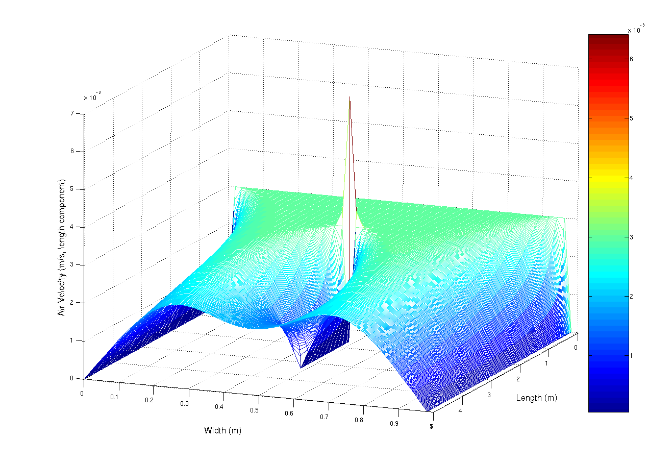
A simulation using the navier-stokes differential equations of the aiflow into a duct at 0.003 m/s (laminar flow). The duct has a small obstruction in the centre that is parallel with the duct walls. The observed spike is mainly due to numerical limitations. This script, which i originally wrote for scilab, but ported to matlab (porting is really really easy, mainly convert comments % -> // and change the fprintf and input statements) Matlab was used to generate the image.
%Matlab script to solve a laminar flow
%in a duct problem

%Constants
inVel = 0.003; % Inlet Velocity (m/s)
fluidVisc = 1e-5; % Fluid's Viscoisity (Pa.s)
fluidDen = 1.3; %Fluid's Density (kg/m^3)

MAX_RESID = 1e-5; %uhh. residual units, yeah...
deltaTime = 1.5; %seconds?
%Kinematic Viscosity
fluidKinVisc = fluidVisc/fluidDen;

%Problem dimensions
ductLen=5; %m
ductWidth=1; %m

%grid resolution
gridPerLen = 50; % m^(-1)
gridDelta = 1/gridPerLen;
XVec = 0:gridDelta:ductLen-gridDelta;
YVec = 0:gridDelta:ductWidth-gridDelta;

%Solution grid counts
gridXSize = ductLen*gridPerLen;
gridYSize = ductWidth*gridPerLen;

%Lay grid out with Y increasing down rows
%x decreasing down cols
%so subscripting becomes (y,x) (sorry)
velX= zeros(gridYSize,gridXSize);
velY= zeros(gridYSize,gridXSize);
newVelX= zeros(gridYSize,gridXSize);
newVelY= zeros(gridYSize,gridXSize);

%Set initial condition

for i =2:gridXSize-1
for j =2:gridYSize-1
velY(j,i)=0;
velX(j,i)=inVel;
end
end

%Set boundary condition on inlet
for i=2:gridYSize-1
velX(i,1)=inVel;
end

disp(velY(2:gridYSize-1,1));

%Arbitrarily set residual to prevent
%early loop termination
resid=1+MAX_RESID;

simTime=0;

while(deltaTime)
 count=0;
while(resid > MAX_RESID && count < 1e2)
 count = count +1;
for i=2:gridXSize-1
for j=2:gridYSize-1
newVelX(j,i) = velX(j,i) + deltaTime*( fluidKinVisc / (gridDelta.^2) * ...
(velX(j,i+1) + velX(j+1,i) - 4*velX(j,i) + velX(j-1,i) + ...
velX(j,i-1)) - 1/(2*gridDelta) *( velX(j,i) *(velX(j,i+1) - ...
velX(j,i-1)) + velY(j,i)*( velX(j+1,i) - velX(j,i+1))));

newVelY(j,i) = velY(j,i) + deltaTime*( fluidKinVisc / (gridDelta.^2) * ...
(velY(j,i+1) + velY(j+1,i) - 4*velY(j,i) + velY(j-1,i) + ...
velY(j,i-1)) - 1/(2*gridDelta) *( velY(j,i) *(velY(j,i+1) - ...
velY(j,i-1)) + velY(j,i)*( velY(j+1,i) - velY(j,i+1))));
end
end

%Copy the data into the front
for i=2:gridXSize - 1
for j = 2:gridYSize-1
velX(j,i) = newVelX(j,i);
velY(j,i) = newVelY(j,i);
end
end

%Set free boundary condition on inlet (dv_x/dx) = dv_y/dx = 0
for i=1:gridYSize
velX(i,gridXSize)=velX(i,gridXSize-1);
velY(i,gridXSize)=velY(i,gridXSize-1);

    end

    %y velocity generating vent
    for i=floor(2/6*gridXSize):floor(4/6*gridXSize)
        velX(floor(gridYSize/2),i) = 0;
        velY(floor(gridYSize/2),i-1) = 0;
    end

%calculate residual for
%conservation of mass
resid=0;
for i=2:gridXSize-1
for j=2:gridYSize-1
%mass continuity equation using central difference
%approx to differential
resid = resid + (velX(j,i+ 1)+velY(j+1,i) - ...
(velX(j,i-1) + velX(j-1,i)))^2;
end
end

resid = resid/(4*(gridDelta.^2))*1/(gridXSize*gridYSize);
fprintf('Time %5.3f \t log10Resid : %5.3f\n',simTime,log10(resid));


simTime = simTime + deltaTime;
end
mesh(XVec,YVec,velX)
deltaTime = input('\nnew delta time:');
end
%Plot the results
mesh(XVec,YVec,velX)
|
| Көнө | 24 февраль 2007 (дата первоначальной загрузки файла на вики) |
| Сығанаҡ | Transferred from en.wikipedia to Commons. |
| Автор | User A1 из английский Википедия |
Лицензиялау
| Был эш авторы User A1 из английский Википедия тарафынан йәмәғәт милекенә ҡулланыуға тапшырылған. Был рөхсәт бөтә донъяла ғәмәлдә. Ҡайһы бер илдәрҙә был хоҡуҡи йәһәттән мөмкин булмауы ихтимал; был осраҡта: User A1 һәр кемгә был эште төрлө маҡсаттарҙа бер ниндә шарттарһыҙ, әгәр улар ҡанун буйынса талап ителмәһә, ҡулланырға рөхсәт итә. |
Төп йөкләүҙәр журналы
The original description page was here. All following user names refer to en.wikipedia.
- 2007-02-24 05:45 User A1 1270×907×8 (86796 bytes) A simulation using the navier-stokes differential equations of the aiflow into a duct at 0.003 m/s (laminar flow). The duct has a small obstruction in the centre that is paralell with the duct walls. The observed spike is mainly due to numerical limitatio
Файл тарихы
Файлдың күрһәтелгән ваҡытта ниндәй өлгөлә булғанын ҡарар өсөн баҫығыҙ: Дата/ваҡыт
| Дата/ваҡыт | Миниатюра | Үлсәмдәре | Ҡатнашыусы | Иҫкәрмә | |
|---|---|---|---|---|---|
| ағымдағы | 16:52, 1 май 2007 | | 1270 × 907 (85 КБ) | wikimediacommons>Smeira | {{Information |Description=A simulation using the navier-stokes differential equations of the aiflow into a duct at 0.003 m/s (laminar flow). The duct has a small obstruction in the centre that is paralell with the duct walls. The observed spike is mainly |
Файл ҡулланыу
Был файлды киләһе бит ҡуллана: